Counting cells using YOLOv5
Contents
Counting cells using YOLOv5
YOLOv5: https://github.com/ultralytics/yolov5
Author of this notebook: Andre Telfer (andretelfer@cmail.carleton.ca)
pip install shapely
Requirement already satisfied: shapely in /home/andretelfer/anaconda3/envs/napari-env/lib/python3.9/site-packages (1.8.2)
Note: you may need to restart the kernel to use updated packages.
import matplotlib.pyplot as plt
import numpy as np
import shapely.geometry
import napari
import pandas as pd

from tqdm import tqdm
from pathlib import Path
from skimage.io import imread, imsave
What does our dataset look like?
Our dataset is just a folder containing .png images of cfos stains
DATA_DIR = Path("/home/andretelfer/shared/curated/brenna/cfos-examples/original")
plt.figure(figsize=(20,20))
sample_image = next(DATA_DIR.glob('*.png'))
image = imread(sample_image)
plt.imshow(image)
<matplotlib.image.AxesImage at 0x7f55958bcf40>
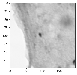
Create a new dataset by sampling sections of the original dataset
SIZE = 200 # size of new images in pixels
SAMPLES_PER_IMAGE = 5

def subsample_image(imagepath, samples):
    image = imread(imagepath)
    h,w,c = image.shape
    locations = np.stack([
        np.random.randint(0,h-SIZE,samples),
        np.random.randint(0,w-SIZE,samples)
    ]).T

    images = []
    for (i,j) in locations:
        new_image = np.zeros(shape=(SIZE,SIZE))
        new_image = image[i:i+SIZE, j:j+SIZE]
        images.append({
            'image': new_image,
            'x': j,
            'y': i,
            'path': imagepath
        })

    return images

sampled_images = []
for image in DATA_DIR.glob('*.png'):
    sampled_images += subsample_image(image, SAMPLES_PER_IMAGE)

plt.imshow(sampled_images[5]['image'])
<matplotlib.image.AxesImage at 0x7f5594517c10>
Save the images to a new directory
OUTPUT_DIR = Path("/home/andretelfer/shared/curated/brenna/cfos-examples/subsamples")

! rm -rf {OUTPUT_DIR}
! mkdir -p {OUTPUT_DIR}

for item in sampled_images:
    image = item['image']
    fname = item['path'].parts[-1].split('.')[0]

    output_file = f"{fname}_{item['x']}x_{item['y']}y.png"
    imsave(OUTPUT_DIR / output_file, image)
ls {OUTPUT_DIR}
Rat2slide1sample3-L_305x_394y.png    Rat2slide1sample4-R_100x_1311y.png
Rat2slide1sample3-L_510x_487y.png    Rat2slide1sample4-R_1367x_1096y.png
Rat2slide1sample3-L_519x_748y.png    Rat2slide1sample4-R_1522x_349y.png
Rat2slide1sample3-L_55x_1035y.png    Rat2slide1sample4-R_1703x_387y.png
Rat2slide1sample3-L_624x_961y.png    Rat2slide1sample4-R_824x_172y.png
Rat2slide1sample3-R_1386x_11y.png    Rat2slide1sample5-L_258x_655y.png
Rat2slide1sample3-R_15x_1024y.png    Rat2slide1sample5-L_496x_1318y.png
Rat2slide1sample3-R_1620x_1176y.png  Rat2slide1sample5-L_693x_447y.png
Rat2slide1sample3-R_44x_328y.png     Rat2slide1sample5-L_705x_749y.png
Rat2slide1sample3-R_582x_896y.png    Rat2slide1sample5-L_79x_700y.png
Rat2slide1sample4-L_1376x_1171y.png  Rat2slide1sample5-R_1320x_1213y.png
Rat2slide1sample4-L_1546x_250y.png   Rat2slide1sample5-R_1474x_655y.png
Rat2slide1sample4-L_1550x_435y.png   Rat2slide1sample5-R_1519x_298y.png
Rat2slide1sample4-L_217x_33y.png     Rat2slide1sample5-R_476x_544y.png
Rat2slide1sample4-L_23x_960y.png     Rat2slide1sample5-R_601x_334y.png
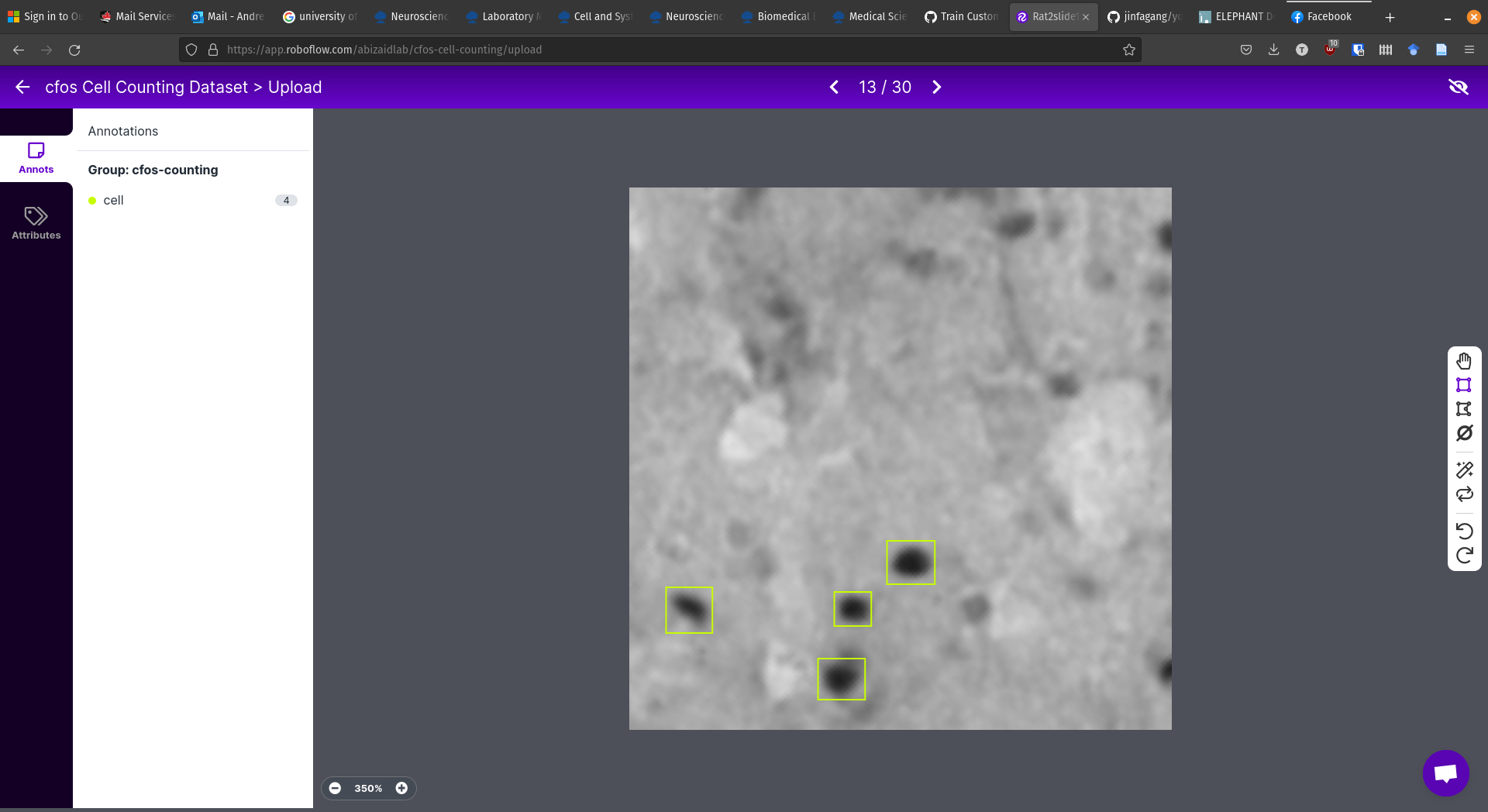
Labeling the Images
For this step, the YOLOv5 documentation recommended roboflow.
I created a free-tier account and started labelling.
I modified the tutorial by not including a scaling preprocessing step. I did this because the size of the cell matters and I wanted to preserve that information
there are some large splotches that are cell shaped, but are not cells
there are small speckles which are not cells
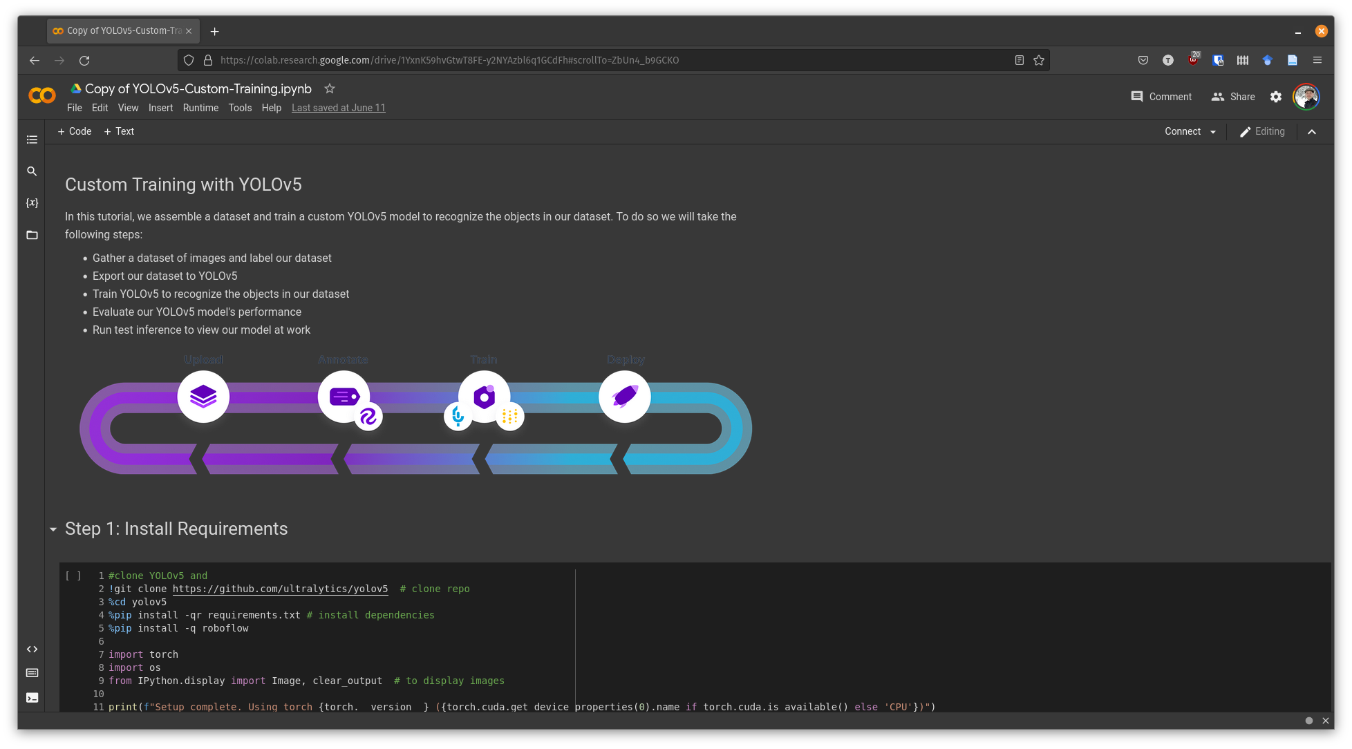
Training a Model
The YOLOv5 guide came with a Google Colab notebook that was easy to modify to my own examples (dataset, image sizes, etc)
Following the guide, I changed the dataset to the one we created in RoboFlow
In order to preserve information about cell size, for training I set the image size to be the same as the actual image size for the sampled training images. When running inference/detection, I used the full image size (e.g. ~2000px in my case).
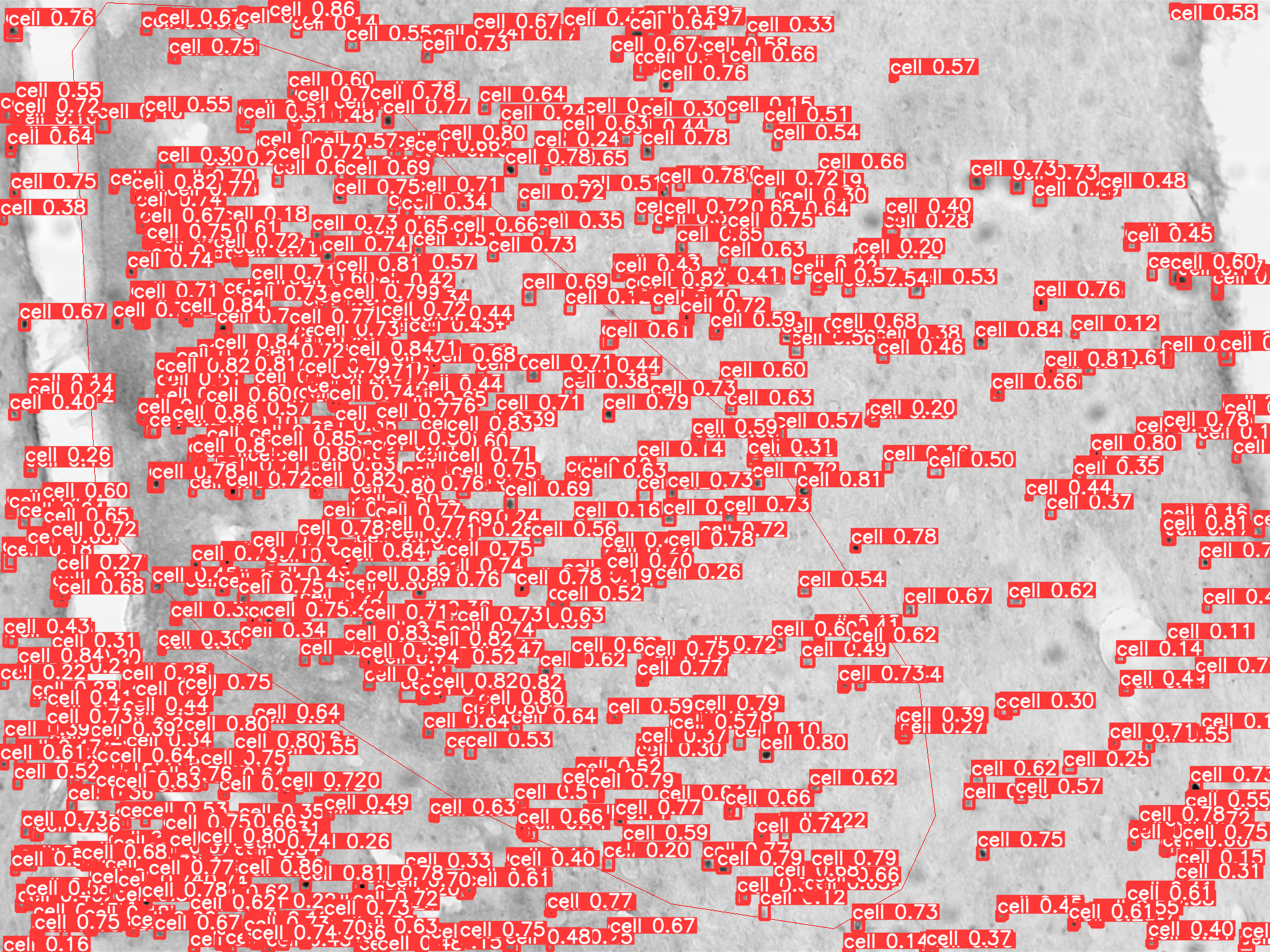
Inference and Results
I uploaded the original images to google drive separately and modified the notebook to use them
The results were overall quite good, although I later found I should’ve labeled more of the lighter cells in the training data; so the model also misses the lighter cells.
Interacting with the results (correcting/viewing)
This will allow us to add/remove cells that were missed
Loading the YOLO labels
all_vertices = []

for idx, p in enumerate(sorted(LABEL_DIR.glob("*.txt"))):
    with open(p, 'r') as fp:
        lines = fp.readlines()

    # Turn the data into a dataframe
    data = [l.strip().split(' ') for l in lines]
    df = pd.DataFrame(data, columns=['0', 'x', 'y', 'w', 'h', 'c']).astype(float)

    # Drop low confidence frames
    df = df[df.c > 0.2]

    # Scale by image size
    fname, _ = p.parts[-1].split('.')
    image = imread(DATA_DIR / f"{fname}.png")
    h, w, c = image.shape
    df.y *= h
    df.h *= h
    df.x *= w
    df.w *= w

    # Get x,y vertices for rectangle
    i = np.ones(shape=df.shape[0])*idx
    vertices = np.array([
        [i, df.y-df.h/2, df.x-df.w/2],
        [i, df.y+df.h/2, df.x-df.w/2],
        [i, df.y+df.h/2, df.x+df.w/2],
        [i, df.y-df.h/2, df.x+df.w/2]
    ]).transpose(2, 0, 1)
    all_vertices.append(vertices)

all_vertices = np.concatenate(all_vertices)
---------------------------------------------------------------------------
NameError                                 Traceback (most recent call last)
Input In [8], in <cell line: 3>()
      1 all_vertices = []
----> 3 for idx, p in enumerate(sorted(LABEL_DIR.glob("*.txt"))):
      4     with open(p, 'r') as fp:
      5         lines = fp.readlines()

NameError: name 'LABEL_DIR' is not defined
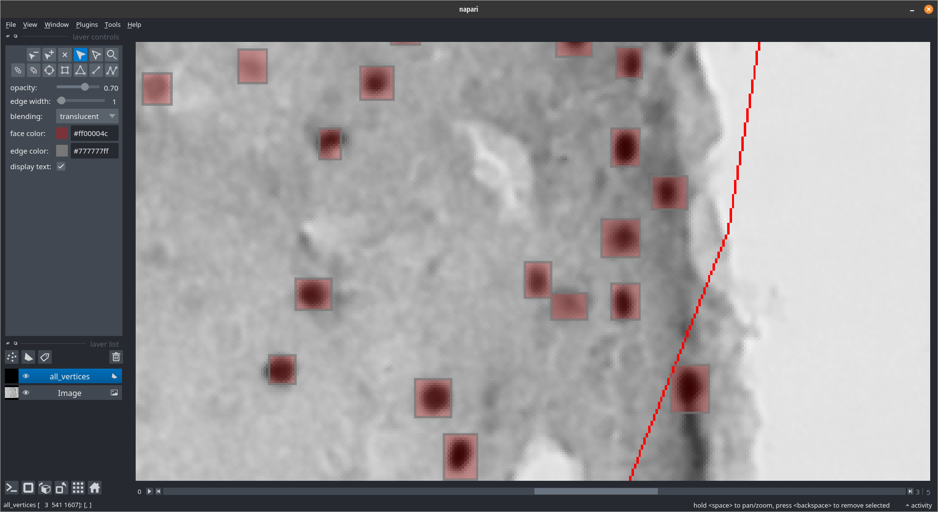
Viewing them with Napari
# The YOLOv5 labels
LABEL_DIR = Path("assets/yolov5-results/labels")

viewer = napari.Viewer()

# Add the images
images = np.array([imread(p) for p in sorted(DATA_DIR.glob("*.png"))])
image_layer = viewer.add_image(np.array(images))

# Add the yolov5 labels
shape_layer = viewer.add_shapes(all_vertices, face_color=[1., 0., 0., 0.3])
Getting cell counts
shape_layer.save('assets/cells.csv')
cells_df = pd.read_csv('assets/cells.csv')
cells_df.head(3)
| index | shape-type | vertex-index | axis-0 | axis-1 | axis-2 | |
|---|---|---|---|---|---|---|
| 0 | 0 | rectangle | 0 | 0.0 | 1041.999713 | 255.000033 |
| 1 | 0 | rectangle | 1 | 0.0 | 1054.999711 | 255.000033 |
| 2 | 0 | rectangle | 2 | 0.0 | 1054.999711 | 264.000031 |
cells_df = cells_df.rename(columns={'axis-0': 'image', 'axis-1': 'y', 'axis-2' : 'x', 'index': 'cell'})
cells_df.head(5)
| cell | shape-type | vertex-index | image | y | x | |
|---|---|---|---|---|---|---|
| 0 | 0 | rectangle | 0 | 0.0 | 1041.999713 | 255.000033 |
| 1 | 0 | rectangle | 1 | 0.0 | 1054.999711 | 255.000033 |
| 2 | 0 | rectangle | 2 | 0.0 | 1054.999711 | 264.000031 |
| 3 | 0 | rectangle | 3 | 0.0 | 1041.999713 | 264.000031 |
| 4 | 1 | rectangle | 0 | 0.0 | 17.000033 | 257.000059 |
Finally, we can get the cell counts for each image
cell_counts = cells_df.groupby('image').apply(lambda x: len(x.cell.unique()))
image
0.0    507
1.0    678
2.0    637
3.0    681
4.0    499
5.0    685
Name: cell_count, dtype: int64
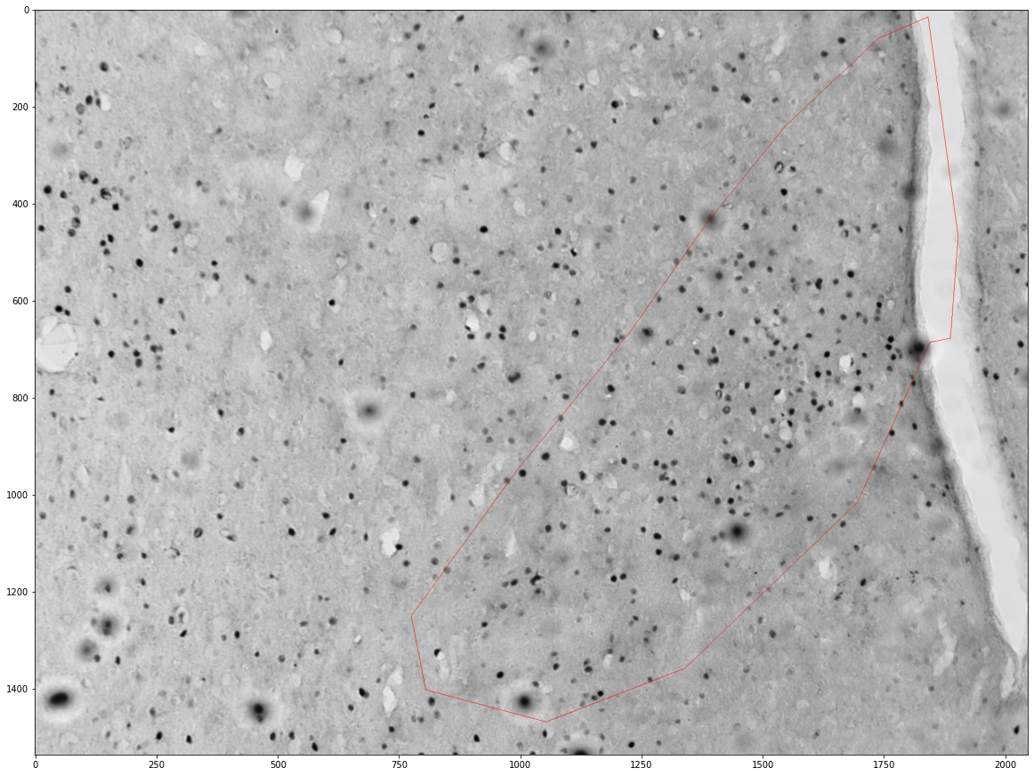
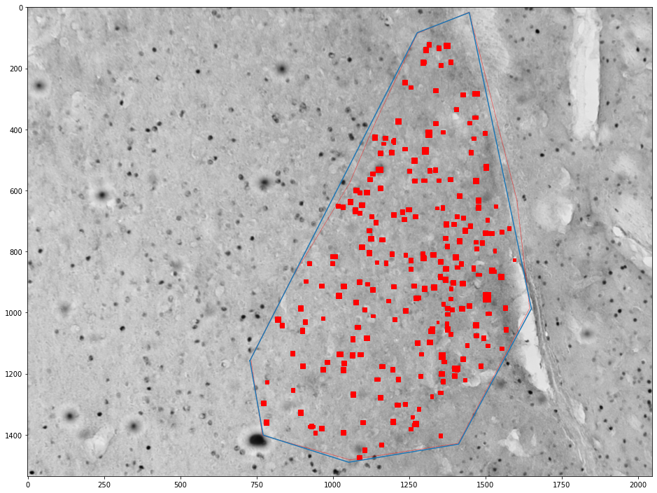
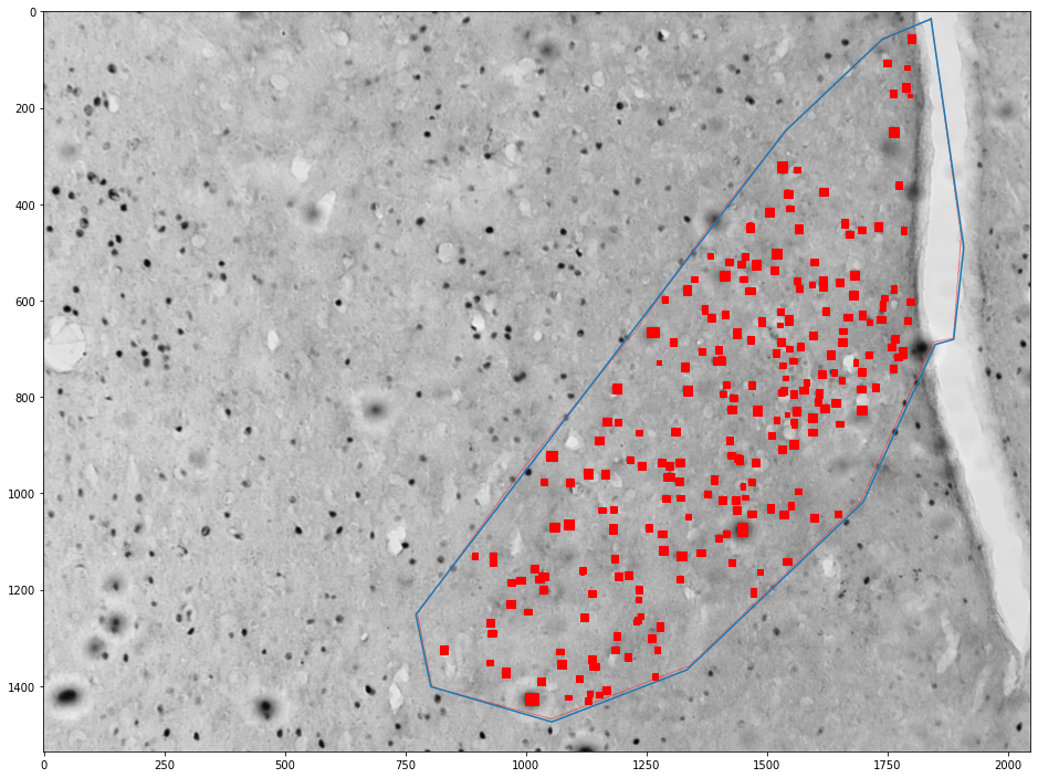
Getting cells in an area
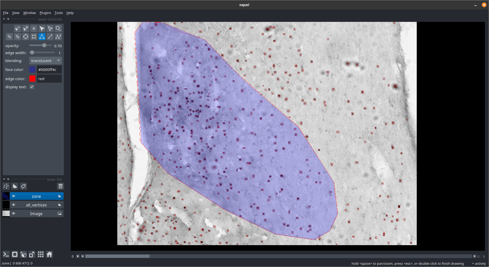
zone_layer = viewer.add_shapes(name='zone', ndim=3, edge_color='red', face_color=[0.,0.,1.,0.3])
zone_layer.save('assets/zones.csv')
zone_df = pd.read_csv('assets/zones.csv')
zone_df = zone_df.rename(columns={'axis-0': 'image', 'axis-1': 'y', 'axis-2' : 'x'})

cells_by_image = cells_df.groupby('image')
zones_by_image = zone_df.groupby('image')

for (idx, zone), (idx, cells) in zip(zones_by_image, cells_by_image):
    zone = shapely.geometry.Polygon(zone[['x', 'y']].values)

    plt.figure(figsize=(16,16))
    plt.imshow(images[int(idx)])
    x,y = zone.exterior.xy
    plt.plot(x,y)
    ax = plt.gca()

    count = 0
    for _, cell in tqdm(cells.groupby('cell')):
        cell = shapely.geometry.Polygon(cell[['x', 'y']].values)
        if zone.contains(cell):
            count += 1
            ax.add_patch(plt.Polygon(np.stack(cell.exterior.xy).T, color='red'))

    plt.show()

    print("Cell count", count)
    print("Density", count / zone.area * 1e6)
    print()
100%|███████████████████████████████████████████████████████████████████████████████████████████████████████████████████████████████████████████████████| 507/507 [00:00<00:00, 2086.06it/s]
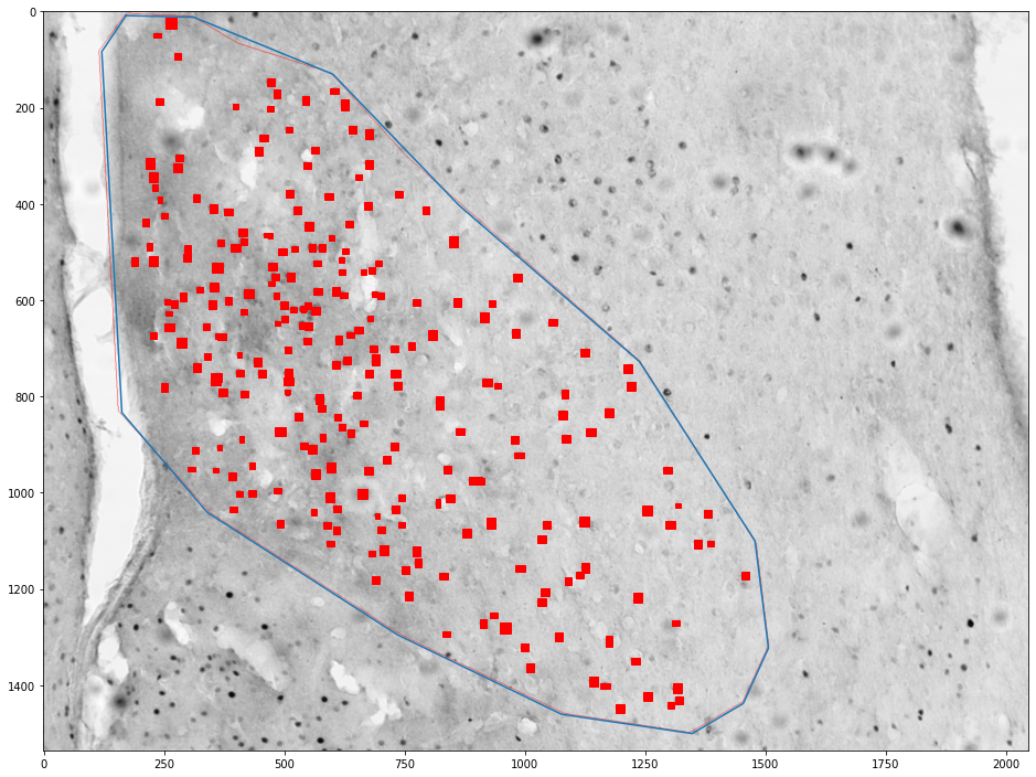
Cell count 253
Density 212.8925598329929
100%|███████████████████████████████████████████████████████████████████████████████████████████████████████████████████████████████████████████████████| 678/678 [00:00<00:00, 2406.08it/s]
Cell count 237
Density 287.37546350839864
100%|███████████████████████████████████████████████████████████████████████████████████████████████████████████████████████████████████████████████████| 637/637 [00:00<00:00, 2235.87it/s]
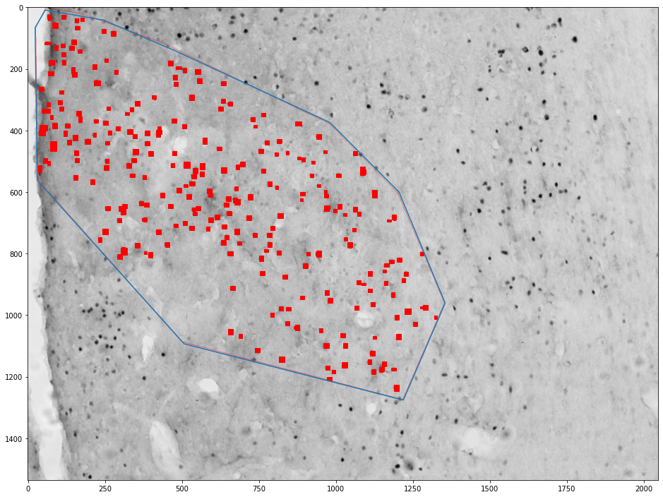
Cell count 280
Density 277.3213753614854
100%|███████████████████████████████████████████████████████████████████████████████████████████████████████████████████████████████████████████████████| 681/681 [00:00<00:00, 2398.25it/s]
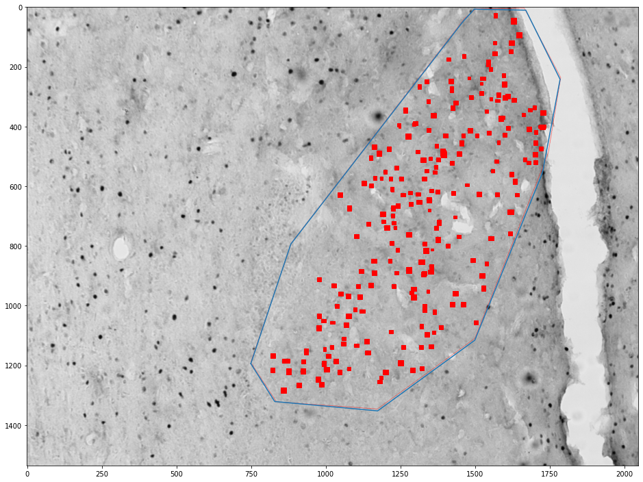
Cell count 231
Density 294.89183180541426
100%|███████████████████████████████████████████████████████████████████████████████████████████████████████████████████████████████████████████████████| 499/499 [00:00<00:00, 2362.33it/s]
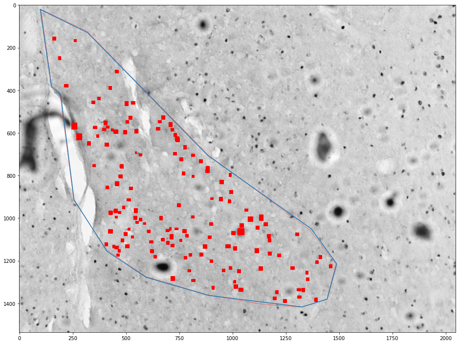
Cell count 155
Density 180.41495343681075
100%|███████████████████████████████████████████████████████████████████████████████████████████████████████████████████████████████████████████████████| 685/685 [00:00<00:00, 2353.12it/s]
Cell count 238
Density 306.52820841199133